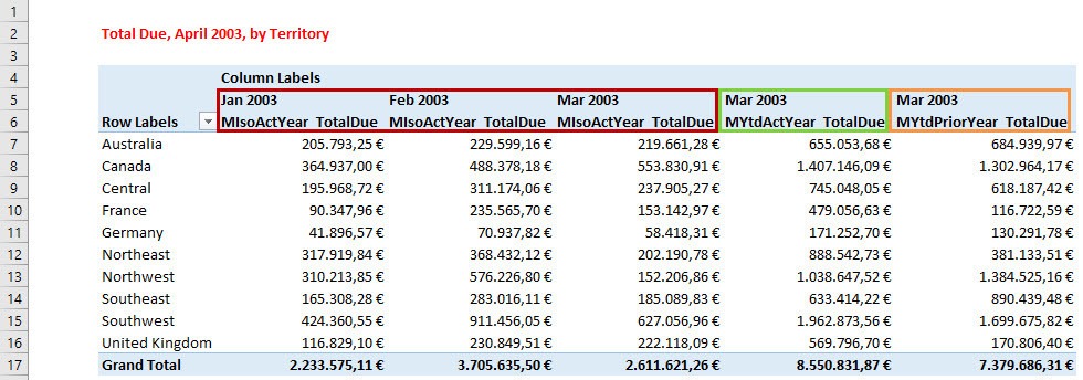
There are many financial reports out there, which have an asymmetric design, to give you all the numbers you need, for a certain place in time. Take a look at the following example to see, what I am talking about. This report gives an overview of Total Due by Territory, for March 2003. The columns in red square represent the single months for year 2003, with its realized Total Due, until March. In green square you see the year-to-date value for 2003, which is the sum of all three single months. In orange you see a year-to-date value again, but this time it’s for the realized Total Due for the same period in the previous year. This is an asymmetric report design and you cannot do this with a „normal“ pivot table. But I have good news for you: You can build asymmetric pivots on Power Pivot data models and I will show you how, in this post.
Why ’normal‘ pivots can’t be asymmetric
When we are talking about asymmetric pivot table design, why is this so special? Can’t normal pivots do that? The answer is: No, they can’t. Take a look at the following screenshot to understand why they can’t.
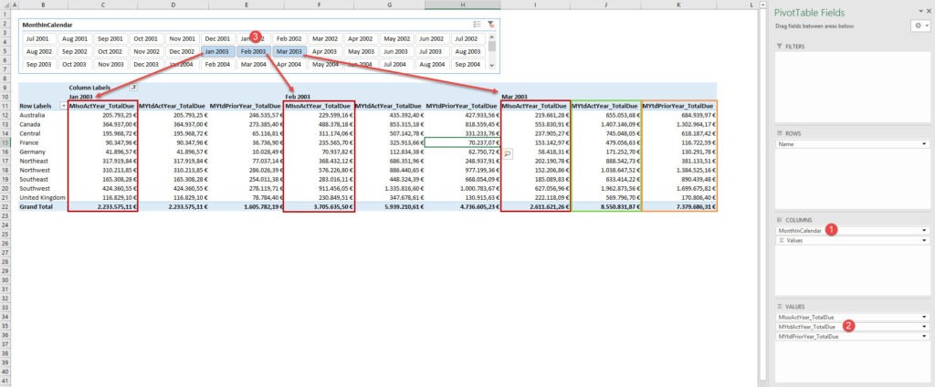
For creating the pivot table above, I did 3 main steps:
- I put MonthInCalendar on columns
- I put the three measures for Total Due on values and
- I filtered MonthInCalendar, so that only Jan 2003 till March 2003 is still active for this pivot table
What does the pivot table do? It creates each combination of the three measures and the three Months from MonthInCalendar and puts it on columns. The result is a report with nine columns, but we only want those in colored squares, which represent the columns from the first screenshot. Or in other words: We want to define, which combination of MonthInCalendar and the choosen measures shall be created.
This is something you can’t do with normal pivots, but you can do this with pivots, that are built on Power Pivot data models. Let’s see how it works.
How you make your pivot asymmetric, working on a Power Pivot data model
There is a way to create asymmetric design, when your pivot is based on a Power Pivot data model (or any other OLAP data source, that can be queried by Multidimensional eXpressions (MDX)). You can build Named Sets to reach this target. Named Sets allow you to define the combination of values and dimension to be shown in the pivot table.
How to create Named Sets via wizard
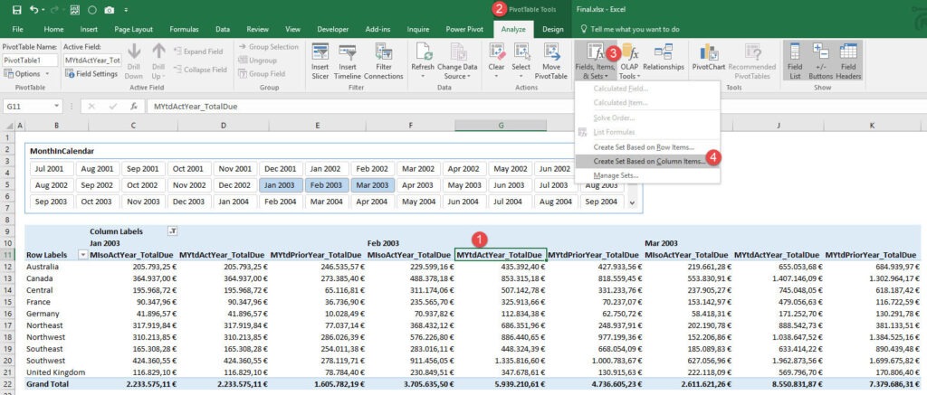
Excel has a nice wizard, which let’s you create your Named Sets quite easy. The next figure shows you the 4 steps to reach the wizard:
- step: Click in the pivot table
- step: Click on the context sensitive menu bar PivotTable Tools
- step: Click on Fields, Items & Sets
- step: Click on Create Set Based on Column Items. It is also possible to create Named Sets based on rows, but this isn’t what we’re going to do here.
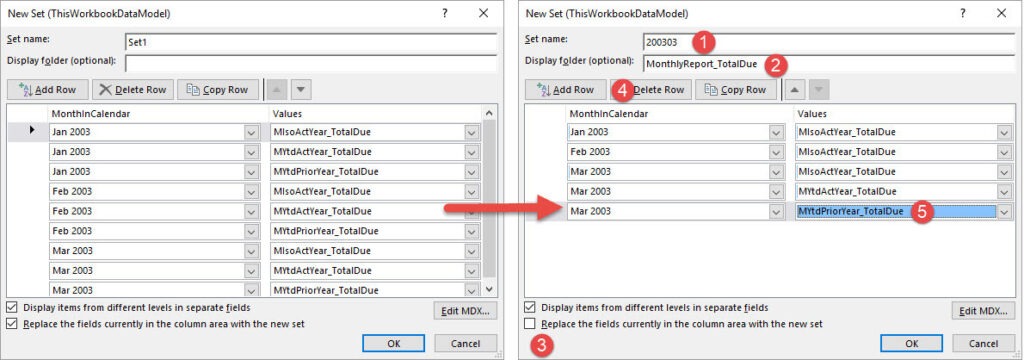
When you reached the wizard, you can create your first Named Set, which means you can create your first defined combination of column headers and values you want. To create your first Named Set follow these steps:
- Step: Give your set a name. If you are preparing a monthly report, I strongly suggest to give it a name like 200303, which stands for March 2003. In a later post I will show you how to control these sets via slicer and therefore this systematic is necessarry.
- Sets can be organized in folders. It’s not mendatory to do so, but I suggest, to organize your Sets in folders like MonthlyReport_TotalDue.
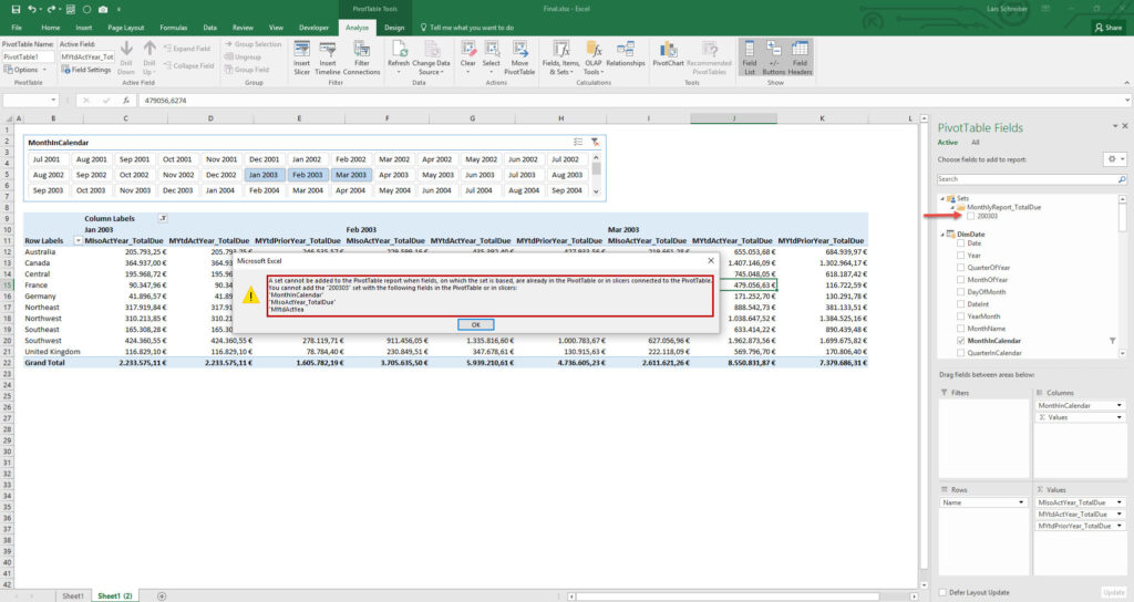
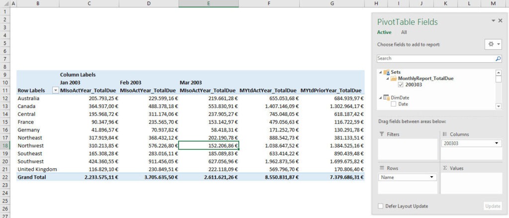
- Step: Uncheck the checkbox Replace the fields currently in the column are with the new set. If you don’t uncheck this box, Excel will throw out the current fields in the pivot and replace it by the newly created set. If you uncheck it here, the set will be created, but not automatically put into the pivot table. You will see later in this post, why this would leed to en error, if you wouldn’t uncheck this checkbox.
- & 5. Step: On the left side of the following figure you see the wizard, when it opens. You see all combinations of MonthInCalendar and Values, that exist in the current pivot table. First delete all the rows you don’t need (we only need 5 columns in the pivot table, so we only need 5 rows in this wizard) and then use the dropdowns, to select which MonthInCalendar and Values you need.
Finding the created Named Set(s) in the pivot table field list
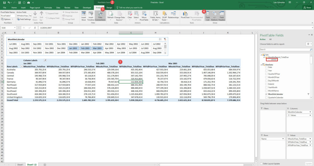
When you are finished with the definition of the Named Set press OK. To find the Named Set in the pivot field list click into the pivot table (1), click on PivotTable Tools (2), click on tab Analyze (3) and Field List (4). Then you will find the newly created Named Set in the Field List, in folder MonthlyReports_TotalDue.
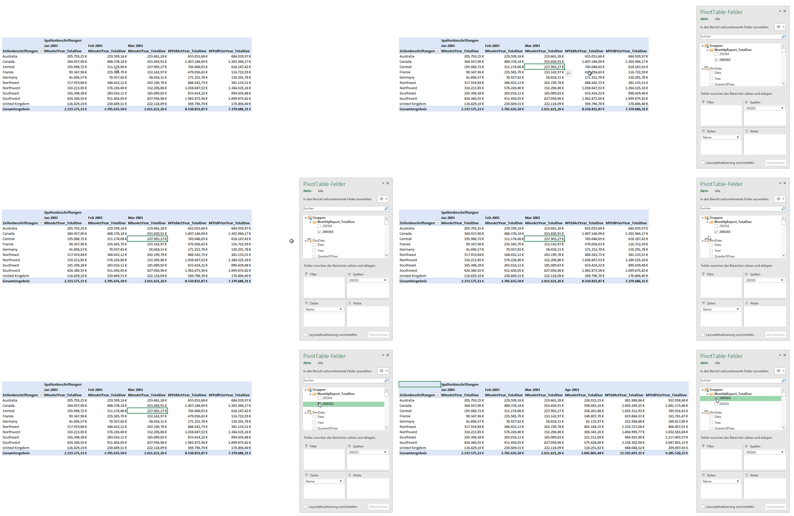
How to use Named Sets in pivot tables
See you next time and keep in mind: Sharing is caring. If you liked this articel, feel free to share it.
Greets from Hamburg,
Lars

Lars ist Berater, Entwickler und Trainer für Microsoft Power BI. Er ist zertifizierter Power BI-Experte und Microsoft Trainer. Für sein Engagement in der internationalen Community wurde Lars seit 2017 jährlich durch Microsoft der MVP-Award verliehen. Lies hier mehr…
